t-Distributed Stochasitc Neighbor Embedding(t-SNE)
논문
Van Der Maaten, Laurens, and Hinton, Geoffrey. “Visualizing data using t-SNE”, Journal of Machine Learning Research (2008).
알고리즘 개선
Poličar, Pavlin G., Martin Stražar, and Blaž Zupan. “Embedding to Reference t-SNE Space Addresses Batch Effects in Single-Cell Classification”, BioRxiv (2019).
속도 개선
Van Der Maaten, Laurens. “Accelerating t-SNE using tree-based algorithms”, Journal of Machine Learning Research (2014).
Linderman, George C., et al. “Fast interpolation-based t-SNE for improved visualization of single-cell RNA-seq data”, Nature Methods (2019).
open t-sNE
필요성
from sklearn.manifold import TSNE 을 통해 작업을 수행하면 "fit_transform" 메서드는 존재하지만 "transform" 메서드는 존재하지 않는다(알고리즘 원리상). 그래서 보통 PCA/SVD, 오토 인코더 등을 사용한다.
Reference
https://stackoverflow.com/questions/59214232/python-tsne-transform-does-not-exist
참고자료
OpenTSNE - 알고리즘이 조금 다르긴 하지만 fit 과 transform 을 따로 수행이 가능하다.
openTSNE is currently the only library that allows embedding new points into an existing embedding.
Reference
https://opentsne.readthedocs.io/_/downloads/en/latest/pdf/
theory
https://opentsne.readthedocs.io/en/latest/tsne_algorithm.html
document
https://opentsne.readthedocs.io/en/latest/api/sklearn.html#openTSNE.sklearn.TSNE.transform
source code
https://opentsne.readthedocs.io/en/latest/_modules/openTSNE/sklearn.html#TSNE
parameter guide
https://opentsne.readthedocs.io/en/latest/parameters.html#parameter-guide
github
https://github.com/pavlin-policar/openTSNE
open t-sNE 설치
Installation - openTSNE requires Python 3.7 or higher in order to run
conda
conda install --channel conda-forge opentsnePyPi
pip install opentsneInstalling from source
https://opentsne.readthedocs.io/en/latest/_modules/openTSNE/sklearn.html#TSNE
python setup.py installoptional
Fast Fourier Transform 을 위해 FFTW3 를 설치하면 더 빠른 연산 가능하고 설치하지 않으면 조금 느리지만 numpy’s implementation of the FFT로 구현이 가능하다.
open t-sNE 예제
iris 자료로 open t-SNE 사용 예제
from sklearn import datasets
from sklearn.model_selection import train_test_split

iris = datasets.load_iris()
X, y = iris["data"], iris["target"]

X_train, X_test, y_train, y_test = train_test_split(X, y, test_size=1/3, random_state=42)

print(X_train.shape, X_test.shape, y_train.shape, y_test.shape)

from openTSNE import TSNE

model = TSNE(verbose=False).fit(X_train)

xtr = model.transform(X_train)
xte = model.transform(X_test)

import matplotlib.pyplot as plt

plt.figure(figsize=(15,10))
plt.scatter(xtr[:,0],xtr[:,1],c=y_train,alpha=0.5,cmap='jet',s=100)
plt.scatter(xte[:,0],xte[:,1],c=y_test,marker="^",alpha=0.5,cmap='cool',s=100)
모델 저장 및 불러오기
import pickle
## Save pickle
with open("tsne.pickle","wb") as fw:
    pickle.dump(model, fw)

## Load pickle
with open("tsne.pickle","rb") as fr:
    load_model = pickle.load(fr)

lmxtr = load_model.transform(X_train)
lmxte = load_model.transform(X_test)
plt.figure(figsize=(15,10))
plt.scatter(lmxtr[:,0],lmxtr[:,1],c=y_train,alpha=0.5,cmap='jet',s=100)
plt.scatter(lmxte[:,0],lmxte[:,1],c=y_test,marker="^",alpha=0.5,cmap='cool',s=100)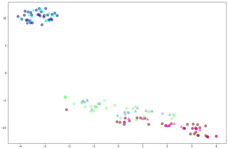
기존 t-SNE 방법을 이용 (결과 비교 참고용)
from sklearn.manifold import TSNE
model = TSNE()
plt.figure(figsize=(15,10))
result = model.fit_transform(X_train)
plt.scatter(result[:,0],result[:,1],c=y_train,alpha=0.5,cmap='jet',s=100)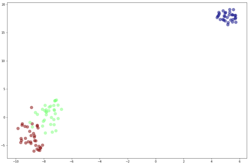
'Study' 카테고리의 다른 글
| GPR Data Labeling - 자체 개발 GUI 개발 및 사용(Upgrade version) (0) | 2023.12.12 |
|---|---|
| GPR Data Labeling - 자체 개발 GUI 개발 및 사용 (0) | 2023.07.14 |
| YOLO - Anchor Boxes Calculation (0) | 2023.07.14 |


